VLOOKUP Function

Function Type: Lookup and Reference

Description:
VLOOKUP is one of the most popular functions in Excel. It is used to lookup a data and retrieve the corresponding data from a specific column. You may either lookup for the exact or approximate match. The "V" in Vlookup means Vertical. It is more frequently used compared to HLOOKUP due to the common database structure we have in Excel.

Function Structure:
=VLOOKUP(lookup_value, table_array, column_index_number, [range_lookup])

Argument Breakdown:
lookup_value - This is the data that excel will lookup into the table. The lookup value should always be in the first column of the table. It may be an alphanumeric, numbers, or a function. There should only be 1 data / cell of lookup value per Vlookup.

table_array - This is the table that excel will lookup into. It should contain the lookup_value. The structure of the table should be in vertical alignment.

column_index_number - This is the relative column number in the table_array. Number 1 corresponds to the leftmost column where the lookup_value is found. Data type for this argument should be number or a function that results to a number value.

[range_lookup] - In this 4th argument, excel is asking us if we are looking into a range in the lookup_value. Argument can be True or False. When we input True, it means approximate match of the lookup_value while False will mean that it will only consider the exact match. 1 can also mean True while 0 or omitting this argument will mean False. The square brackets means this argument is optional.

Example:

These are examples of Vlookup.

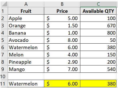
Supposed we want to search the price and available QTY dynamically based on the name of the Fruit.

The functions will be:
B11 =VLOOKUP(A11,A1:C9,2,FALSE)
To populate the Price in B11, we look up the name of the Fruit of A11 in the range A1:C9 and return the value from 2nd column.

C11 =VLOOKUP(A11,A1:C9,3,FALSE)
To populate the Available QTY in B11, we look up the name of the Fruit of A11 in the range A1:C9 and return the value from 3rd column.

Notice the difference? They only differ in their 3rd argument which is the column_index_number. The Price used 2 because it was in the 2nd column of the table while Available QTY used 3 because it was in the 3rd column.

Three main limitation in VLOOKUP:
1.As mentioned above, the lookup value must be in the first column of a VLOOKUP table range

2.Excel will always return the value from the top most row of a table range when multiple instances of the lookup value are present.

Pro tip: Make sure to use unique names/IDs in the first column to avoid missing the other lookup value rows.

3.We can't lookup images.

---

Still need help with Excel and Google Sheets?
Get Instant Expert Help
We can also accept LEO, HIVE, HBD tokens as payment.

---

This post is designated as a reviewer for Excel trainings I conduct.

Feel free to share with anyone. 😉

Earnings from Upvotes on this post are used to continue sharing Excel knowledge.
If you also want to earn HIVE in 7 days while blogging your favorite topics, join us here at Peakd.
*Thumbnail used is made in Canva.