In exercise 63 of section I.3 of Larson's Calculus with Analytic Geometry Volume I on page 68 on the topic of limits and their properties, use a software or program to graph the function and estimate the limit. Use a table to support the conclusion. Then calculate the limit using analytical methods.

To graph the function and estimate its limit, we would say that the function is:

Its graph using Geogebra software is:
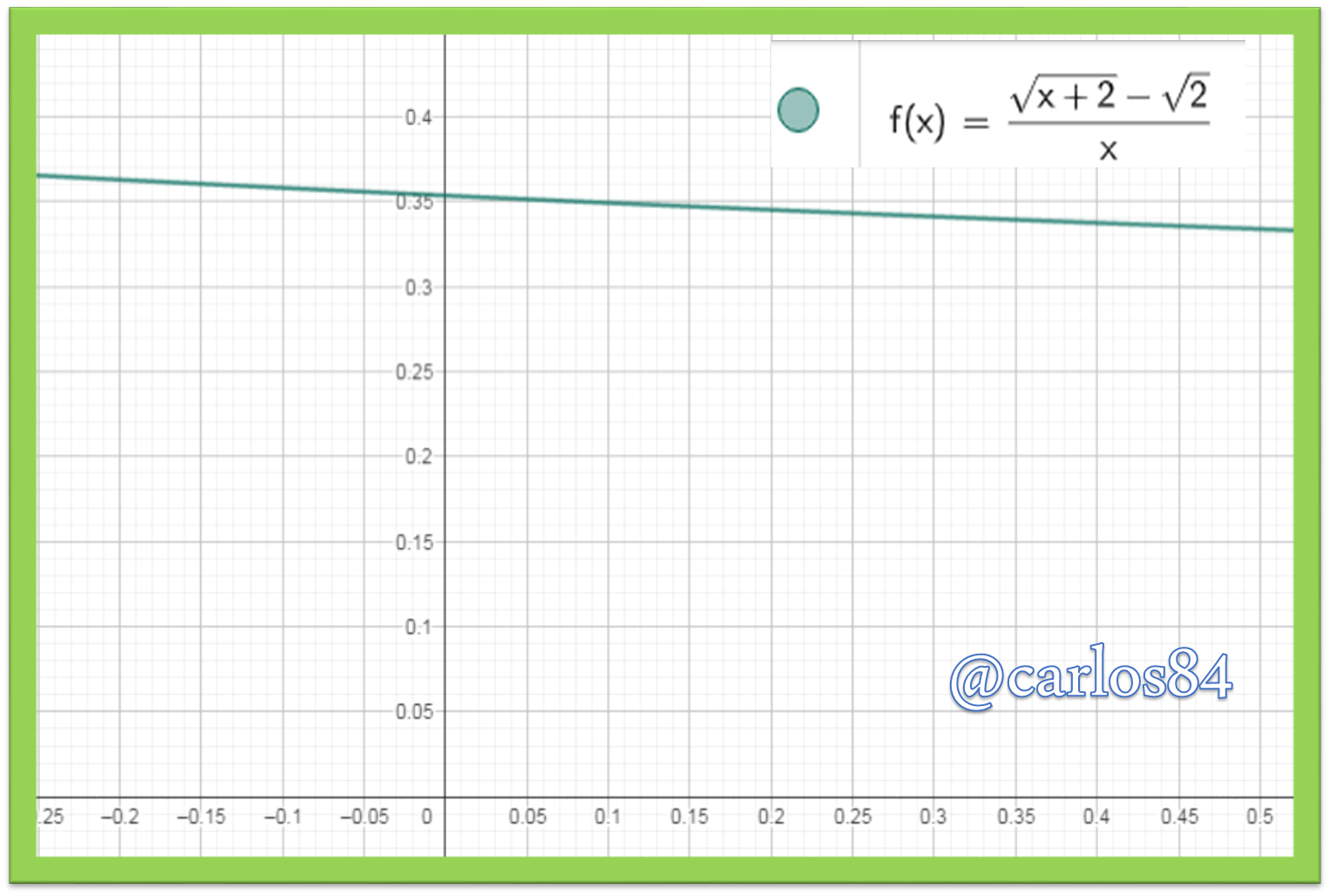
As the function cuts the y-axis at about 0.35, then I would estimate that the limit of the function when x tends to zero is 0.35, however we still need to support this result with a table:
Before that we calculate the images of the function for values approaching zero on the right and on the left:

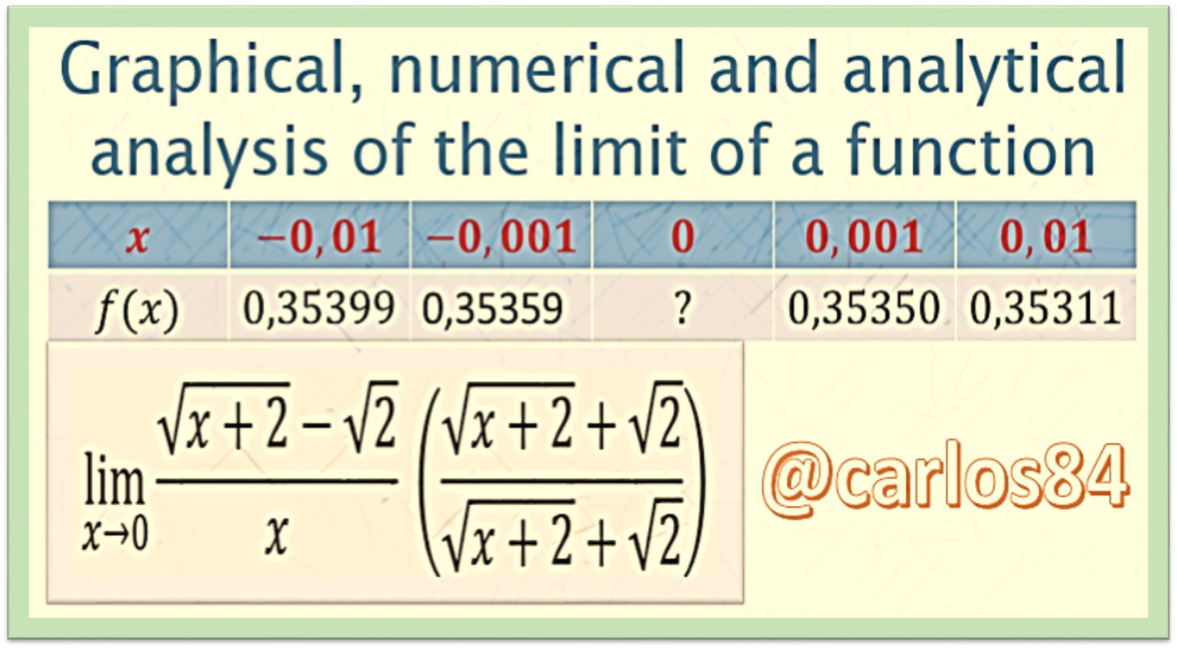
Finally, the table is:
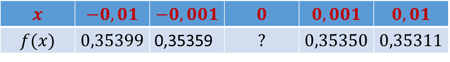
The approximation of the values of x when it tends to zero on the right and on the left leads us to conclude that the value of the limit is 0.35.
Use an analytical method to solve for the limit
The most convenient analytical method is the conjugate method, which is a rationalization method that consists of multiplying the numerator up and down by simply changing the sign, as follows:

We multiply numerator with numerator and denominator with denominator:

Conclusion
As we could see in the development of this post, by means of the graph of the function we can estimate the limit of a real function using software or some program for graphing. Making a table of values to find the images of the values of x that approach zero on the left and on the right and applying an algebraic technique of rationalization, we could reach the same conclusion, i.e. that the value of the limit of the rational function proposed in this post is 0.35.