My goal with this article is to help you enhance your Excel skills and save time for yourself. I would like to share some of the tricks and techniques I use to save time when working with formulas. The compound time-saving effect can make a big difference to our work setting allowing us to spend our earned time to other things important to us.

Most of us spend a lot of time working with formulas, and it’s not always a smooth process. As you advance, your formulas get more complicated and time-consuming to maintain. This is the environment of Excel, it can do some amazing calculations with limitless potential, but this means it can also get really messy.
I like to explore the fastest and most effective approach to accomplish a task, and this article includes my top 10 techniques that help me be more productive.
- AutoSum Alt+= keyboard shortcut
- F2 & Esc keyboard shortcuts
- Using Ctrl key for multiple cell references
- Being aware of enter and edit modes
- Taking advantage of the function screen tip
- Quickly jump to a cell reference with F5
- Using the Functions Argument
- Expanding the formula bar
- Understanding Structured References
- Using Trace Dependents before deleting
These Excel features, functions, keyboard shortcuts, and techniques I use nearly every day. If you are an Excel user, I encourage you to pick some of these up If you haven't already to save up some time.
1# AutoSum Alt+=
The one formula I use the most frequently is the SUM function. And the quickest way to create a sum formula is to have Excel do it for you.
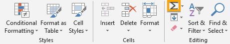
The AutoSum button (found on the Home tab and Formulas in the Ribbon) will automatically create a sum formula for a row or column of numbers. The button is only on the Formulas tab on the Mac.
The keyboard shortcut for AutoSum is Alt+= (hold down the Alt key, then press the “=” key). The shortcut on the Mac is Command+Shift+
Ways to use it:
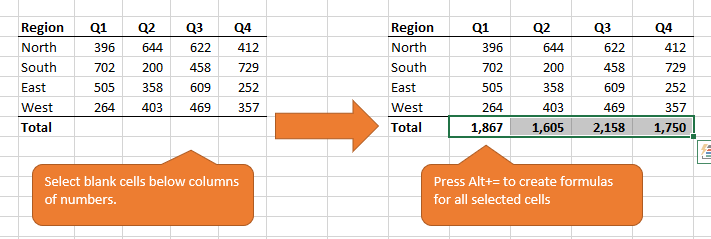
- Simply select a blank cell underneath a column of numbers or to the right of a row of numbers then click the AutoSum button.
- You can also select all the cells in a row/column that contain numbers, then click the AutoSum button. The sum formula will be created in the first blank cell directly underneath to the selection.
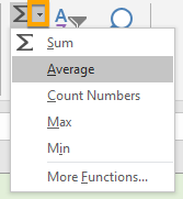
- By selecting the drop-down arrow to the right of the AutoSum button gives you options to create formulas with other functions such as Average, Count, Min, Max.
- Create formulas in multiple cells at the same time by selecting a row of blank cells below your data and press Alt+=. The sum formulas will be created in all of the blank selected cells that are below a column or to the right of a row of numbers. This makes creating the formulas even faster.
2# F2 & Esc keys
Once a formula is written, I tend to spend a lot of time editing and revising it. This is especially true when I'm working on someone else’s file and learning what their formulas calculate. This is where the F2 and Escape keys on the keyboard can really save my time.
How to use it:
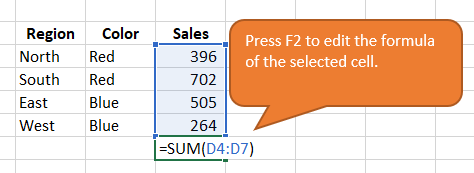
- For editing, just select any cell that contains a formula and press the F2 key. This opens the formula for editing directly in the cell, without having to use the mouse. The F2 equivalent on the Mac is Ctrl+U.
You can now use the left and right arrow keys on the keyboard to move with the cursor and edit, add, or delete text as needed.
- For auditing, press the F2 key on the cell containing the formula and see what cells are being referenced in the formula with the help of the colored boxes.
In the example below, I can easily see that the SUMIFS formula is returning an error because the rows are not extending down the same amount of as the other arguments in the formula.
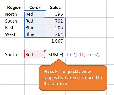
- The Escape [Esc] key exits the formula edit mode without changing the formula. This allows you to instantly review the formula and its references with the F2 key, then press the Escape key if you do not need to do changes.
3# Quickly add multiple Cell References
Often times you will need to calculate cells in a range which is not joined together. The image below shows an example of this.
I need to create a formula that sums the Total rows for each product.
The SUM formula for the Grand Total should be
=SUM(C9,C13,C17).
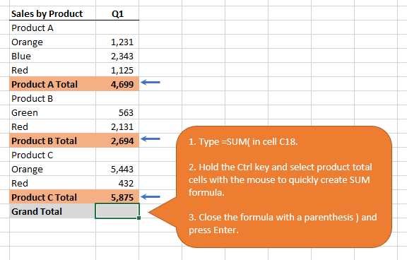
The problem is that typing this formula can take considerable time and be more prone to a mistake, particularly if you have a lot of subtotal rows to sum up. The fastest way to produce this formula is to hold down the Ctrl key and select the cells you want to include by left-clicking the cells with the mouse.
Step by step how to use it:
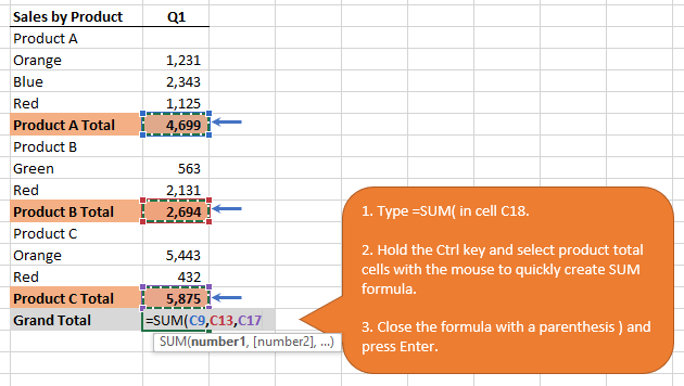
- Type =SUM( in cell C18 to start the formula.
- Hold down the Ctrl key on the keyboard.
- Left-click cell C9 with the mouse.
- Continue to keep the Ctrl key held down and left-click on cell C13
- Formula now reads: =SUM(C9,C13
- Continue to left-click additional cells to add them to the formula
- When finished, close the formula with a parenthesis )
- Click Enter on the keyboard to enter the formula.
4# Awareness of enter and edit modes
I remember dealing with the frustrating moments and wondering why is that while editing a formula and moving the cursor left/right, instead of the navigating the courser in the formula section, a new cell reference is inserted in the formula?
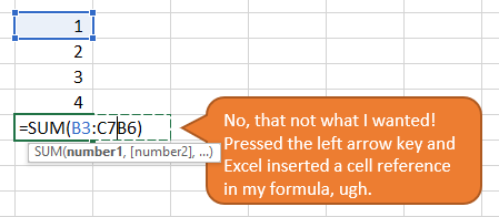
Later I found out that this behavior is made by the different formula mode that Excel is in when I'm editing the formula in the cell.
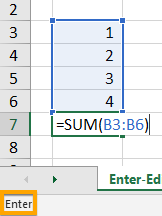
There are two different modes that Excel can be: Edit & Enter.
Edit Mode – Excels default mode. In this environment, we can use the left and right arrow keys to navigate the cursor within the formula and make changes.
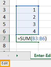
Enter Mode – Enter mode is used for referencing cells or ranges in your formula. Clicking the arrow keys on the keyboard will choose cells in the worksheet and add to the selected cell in the formula. This is the mode that can be annoying if you are just trying to move the cursor within your formula.
How to use it:
Pressing the F2 key will toggle between Edit and Enter modes, giving you more control over your formulas. The F2 equivalent on the Mac is Ctrl+U.
This entry mode applies to other features in Excel where you need to choose a group of cells, for example, changing the source data for a chart or PivotTable.
5# Taking Advantage of the Function Screen Tip
The truth is that the function ScreenTip is Packed with Features and a lot of people don't use it to the full extent.
I talking about this small box that appears under the formula bar or cell when you are editing a formula.
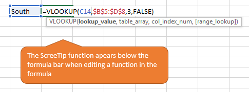
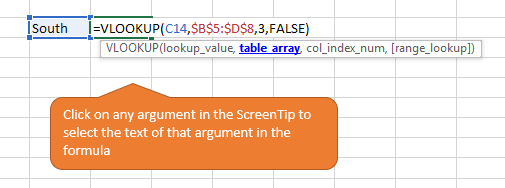
The part in the function that you are editing will be displayed in bold in the ScreenTip.
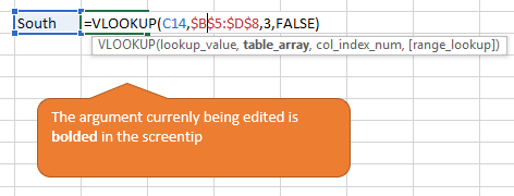
You can click on any of the argument in the ScreenTip box to select the text of that argument. This way you can navigate within the formula much quicker and reduce the possibility of making errors.
For what can it be used:
I can click “table_array” in the ScreenTip box with my mouse and the corresponding part in the formula will be selected. It is much quicker in comparison trying to select the text using the mouse cursor.
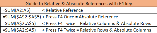
The ScreenTip link can further be used to quickly change the cell reference between absolute and relative. For the F4 key to work, the cursor must be placed inside the reference or the cell reference must be selected.
After you selected the argument, press F4 on the keyboard (Command+T on Mac). This adds the $ symbol in front of the column letter and row number to anchor the reference.
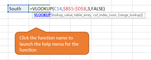
- By Selecting the Function name in the box will launch the help menu or open the support page URL where you can read and watch videos about the function. A quick way to learn more about formulas and functions we encounter without the need for going searching on the internet.
- If your formula is long and wrapping below and it's in your way, you can move it. Just cover the left side of the ScreenTip with your mouse until the cursor changes to the cross icon. Left click and hold it, this way you can drag it to a new location.
6# Quickly jump to a cell reference with F5
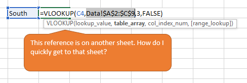
There are many occasions when I have to navigate within my workbook to find a cell or range that is on another worksheet and the following tip is saving me a lot of time.
Step by Step what you can do:
- Use the ScreenTip to quickly select a cell or range that is referenced in a formula
- Press F5 key (Ctrl+G on Mac) on the keyboard to the Go To menu.
- Press OK on the Go To menu
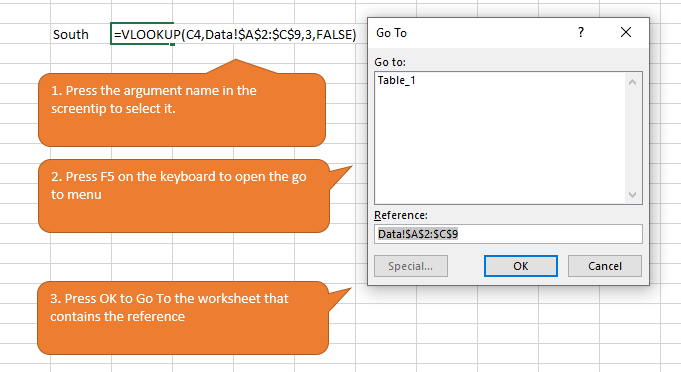
- Reference (Data) will be activated and the range will be selected on the corresponding workbook. From there you can quickly view and change the range in the formula.
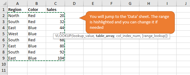
Navigating through workbook is not a hustle anymore. You don't have to waste time going into worksheets to find the ranges that are referenced in the formulas.
7# Using the Functions Argument
The Functions Argument Window can give you detailed information about a function in your formula. It can save you time when trying to audit a function, to see what is included in the formula in a way that won’t make your head spin.
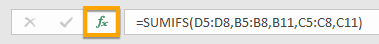
Selecting the cell with the reference and click the formula icon to the left of the formula bar. The quickest way to open it is with the keyboard shortcut, Shift+F3 (Ctrl+A on Mac).
When to use it:
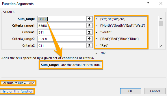
The Function Arguments Window can be used to displays all the arguments in the function in an organized way. This is a simple way to inspect the longer function.
The window also presents the definition of the selected argument. This is helpful when you are learning the functions and not sure what is expected for each argument of the function. You can also click on “Help on this function” link in the bottom left corner to open the full help menu and learn more about the function.
Note: the Same function on Mac is called the Formula Builder. It is laid out a little differently than what I presented here, but it has the same features and should be helpful.
8# Expanding the formula bar
When your formula gets very long, you can expand the height of the Formula Bar. This a simple quick tip, but it can be really helpful when viewing large formulas.

How to expand the formula bar:
In the image above I have an example of a long formula. I can increase the height of the bar to view the entire formula by hovering the mouse over the bottom of the formula bar until the cursor turns to vertical arrows. Then left-click and drag the bar down to make it taller.
The quickest way to automatically expand/collapse the formula bar is using the keyboard shortcut Ctrl+Shift+U (same on the Mac). This keyboard shortcut is especially useful if you are working on a laptop and you want to view as much of the grid as possible. It allows you to quickly collapse the formula bar when you’re not working on a long formula.
9# Understanding Structured References
Excel Tables were designed to save time for the user when working with data and I think they do a very great job of it.
What were previously time-consuming tasks like the styling, sorting, filtering, summarizing and rearranging our data, now become extremely quick and easy with Tables.
A separate article should be written on the topic of Excel Tables, cause it has many great features, one particularly nice feature of the Tables is the new formula syntax called Structured References.
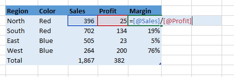
As you can see in the image below, the structured reference syntax uses column names instead of cell addresses. If this cell was not in a table, the formula would read =E5/D5
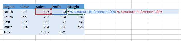
It uses the names of the columns of the table, eliminating the need to include the sheet name in the formula to reference a range. This makes formulas much simpler to read and write.
It has its learning curve and some getting used to, but in the long run, you will save a lot of time using tables.
10# Using Trace Dependents before deleting
Have you ever been in a situation where you needed to delete an entire sheet, but you were afraid that some formulas depend on it and don’t want your model to blow up? This is a common problem, especially when you are receiving a project from someone else and you don't know how it was built.
Trace Dependents feature can help you out in these situations. Before you delete the sheet, you should trace the dependents of cells that might be used by different sheets in the workbook.
Example:
We have a VLOOKUP formula on ‘Sheet1’ that references the ‘Data’ sheet.
=VLOOKUP(A1,Data!$B$2:$D$100,2,False)
If you delete the ‘Data’ sheet then this formula on ‘Sheet 1’ will return an error.
To prevent this you need to trace the dependent formulas of the cells on the ‘Data’ sheet to see what formulas rely on them and it is used in the following way:
Choose a cell that possibly contains references in a formula located on a different sheet, then press the Trace Dependents button on the Formulas tab in the ribbon. The keyboard is Alt+T+U+D (Ctrl+ on Mac). The keyboard shortcut to remove the trace arrows is Alt+T+U+A (Ctrl+ on Mac).
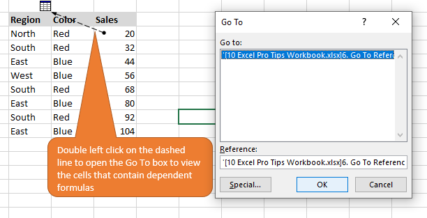
If the Trace Dependents function detects entries in other sheets that depend on the chosen formula, a dashed arrow will appear with a spreadsheet icon. Notice the image below.
By double-clicking on the black arrow line you will be sent to the Go To box. (Make sure you click on the black dashed line between the selected cell and the spreadsheet icon to get the Go To box.)
Once it's open, you can choose any entry in the list to Go To that specific cell. Then you can audit the formula and decide if it is still needed or not.
11# Bonus Tip: Learn a new function every day
I hope that you gained some useful tips from these mentioned techniques. There is constantly something new we can learn in Excel, and that is what makes it enjoyable and challenging to work with at the same time.
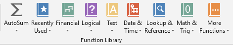
As a bonus tip, I would encourage you to continue learning more about Excel functions whenever you are able to and a great way to go to the Formulas tab in the ribbon, click on any of the Function drop-down buttons, hover the mouse over a function you are not familiar with, and press F1 on the keyboard to launch the Excel help menu and there you can search and read about the function while simultaneously testing it out on the worksheet. You are going to be amazed at what you learn!
This post has received a 6.11 % upvote from @boomerang.
Congratulations @exgap! You have completed the following achievement on the Steem blockchain and have been rewarded with new badge(s) :
Click here to view your Board
If you no longer want to receive notifications, reply to this comment with the word
STOPTo support your work, I also upvoted your post!
You got a 9.94% upvote from @minnowvotes courtesy of @exgap!