Learn Python Series (#31) - Data Science Part 2 - Pandas
![]()
Repository
What will I learn?
- You will learn how to convert date/datetime strings into
pandasTimestamps, and set those Timestamp values as index values instead of default integer numbers which don't provide useful context; - how to slice subsets of TimeSeries data using date strings;
- how to slice time-based subsets of TimeSeries data using
.between_time(); - how to return and use some basic statistics based on common
pandasstatistical methods.
Requirements
- A working modern computer running macOS, Windows or Ubuntu;
- An installed Python 3(.7) distribution, such as (for example) the Anaconda Distribution;
- The ambition to learn Python programming.
Difficulty
- Beginner
Curriculum (of the Learn Python Series):
- Learn Python Series - Intro
- Learn Python Series (#2) - Handling Strings Part 1
- Learn Python Series (#3) - Handling Strings Part 2
- Learn Python Series (#4) - Round-Up #1
- Learn Python Series (#5) - Handling Lists Part 1
- Learn Python Series (#6) - Handling Lists Part 2
- Learn Python Series (#7) - Handling Dictionaries
- Learn Python Series (#8) - Handling Tuples
- Learn Python Series (#9) - Using Import
- Learn Python Series (#10) - Matplotlib Part 1
- Learn Python Series (#11) - NumPy Part 1
- Learn Python Series (#12) - Handling Files
- Learn Python Series (#13) - Mini Project - Developing a Web Crawler Part 1
- Learn Python Series (#14) - Mini Project - Developing a Web Crawler Part 2
- Learn Python Series (#15) - Handling JSON
- Learn Python Series (#16) - Mini Project - Developing a Web Crawler Part 3
- Learn Python Series (#17) - Roundup #2 - Combining and analyzing any-to-any multi-currency historical data
- Learn Python Series (#18) - PyMongo Part 1
- Learn Python Series (#19) - PyMongo Part 2
- Learn Python Series (#20) - PyMongo Part 3
- Learn Python Series (#21) - Handling Dates and Time Part 1
- Learn Python Series (#22) - Handling Dates and Time Part 2
- Learn Python Series (#23) - Handling Regular Expressions Part 1
- Learn Python Series (#24) - Handling Regular Expressions Part 2
- Learn Python Series (#25) - Handling Regular Expressions Part 3
- Learn Python Series (#26) - pipenv & Visual Studio Code
- Learn Python Series (#27) - Handling Strings Part 3 (F-Strings)
- Learn Python Series (#28) - Using Pickle and Shelve
- Learn Python Series (#29) - Handling CSV
- Learn Python Series (#30) - Data Science Part 1 - Pandas
Additional sample code files
The full - and working! - iPython tutorial sample code file is included for you to download and run for yourself right here:
https://github.com/realScipio/learn-python-series/blob/master/lps-031/learn-python-series-031-data-science-pt2-pandas.ipynb
I've also uploaded to GitHub a CSV file containing all actual BTCUSDT 1-minute ticks on Binance on dates June 2, 2019, June 3, 2019 and June 4, 2019 (4320 rows of actual price data, datetime, open, high, low, close and volume), which file and data set we'll be using:
https://github.com/realScipio/learn-python-series/blob/master/lps-031/btcusdt_20190602_20190604_1min_hloc.csv
GitHub Account
Learn Python Series (#31) - Data Science Part 2 - Pandas
Welcome to episode #31 of the Learn Python Series! In the previous episode (Learn Python Series (#30) - Data Science Part 1 - Pandas) I've introduced you to the pandas toolkit, and we've already explained some of the basic mechanisms. In this episode (which is no.2 of the Data Science sub-series, also about pandas) we'll expand our knowledge using more techniques. Let's dive right in!
Time series indexing & slicing techniques using pandas
Analysing actual BTCUSDT financial data using pandas
First, let's download the file btcusdt_20190602_20190604_1min_hloc.csv found here on my GitHub account, and save the file to your current working directory.
Next, let's open the file like so:
import pandas as pd
df = pd.read_csv('btcusdt_20190602_20190604_1min_hloc.csv')
df.head()
| open | high | low | close | volume | datetime | |
|---|---|---|---|---|---|---|
| 0 | 8545.10 | 8548.55 | 8535.98 | 8537.67 | 17.349543 | 2019-06-02 00:00:00+00:00 |
| 1 | 8537.53 | 8543.49 | 8524.00 | 8534.66 | 31.599922 | 2019-06-02 00:01:00+00:00 |
| 2 | 8533.64 | 8540.13 | 8529.98 | 8534.97 | 7.011458 | 2019-06-02 00:02:00+00:00 |
| 3 | 8534.97 | 8551.76 | 8534.00 | 8551.76 | 5.992965 | 2019-06-02 00:03:00+00:00 |
| 4 | 8551.76 | 8554.76 | 8544.62 | 8549.30 | 15.771411 | 2019-06-02 00:04:00+00:00 |
df.shape
(4320, 6)
A quick visual inspection of this CSV file (using .head(), and .shape) shows that we're dealing with a data set consisting of 4320 data rows, and 6 data columns, being datetime, open, high, low, close, and volume.
Nota bene: This data set contains actual trading data of the BTC_USDT trading pair, downloaded from the Binance API, sliced to only contain all 1 minute k-lines / candles on (the example) dates 2019-06-02, 2019-06-03, and 2019-06-04, which I then pre-processed especially for this tutorial episode. The original data returned by the Binance API contains timestamp values in the form of "epoch millis" (milliseconds passed since Jan 1st 1970), and I've converted them into valid ISO-8601 timestamps, which can be easily parsed by the pandas package, as we'll learn in this tutorial.
Using the Jupyter Notebook / iPython %matplotlib inline Magic operation, let's take a look how the spot price of Bitcoin has developed minute by minute on these dates, by plotting the df['open'] price values:
%matplotlib inline
df['open'].plot()
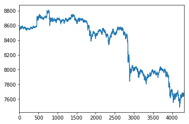
<matplotlib.axes._subplots.AxesSubplot at 0x1211f5f28>
Datetime conversion & indexing (using .to_datetime() and .set_index() methods)
The pandas library, while converting the CSV data to a DataFrame object, by default added numerical indexes.
The visual plot example showing the open prices per minute just now, contains X-asis values coming from the numerical indexes that pandas set for now. Although it is clear we're in fact plotting 4320 opening price values, those numbers don't provide any usable context on when the price of Bitcoin was developing over time.
Because we're working with time series now, it would be convenient to be able to set and use the timestamps in the "datetime" column as index values, and to be able to plot those timestamps for visual reference as well.
But if we inspect the data type of the first timestamp (2019-06-02 00:00:00+00:00), by selecting the "datetime" column and the first row (index value 0), like so, we discover that value is now of the string data type:
type(df['datetime'][0])
str
We can convert all "datetime" column values (in one go, with a vectorised column operation) from string objects to pandas Timestamp objects, using the pandas method .to_datetime():
df['datetime'] = pd.to_datetime(df['datetime'])
type(df['datetime'][0])
pandas._libs.tslibs.timestamps.Timestamp
Next, we can re-index the entire DataFrame to not use the default numerical index values, but the converted Timstamp values instead. The .set_index() method is used for this, and calling it will not only use the Timestamps as index values, therewith unlocking a plethora of functionalities, but .set_index() will also remove the 'datetime' column from the data set:
df = df.set_index('datetime')
df.head()
| open | high | low | close | volume | |
|---|---|---|---|---|---|
| datetime | |||||
| 2019-06-02 00:00:00+00:00 | 8545.10 | 8548.55 | 8535.98 | 8537.67 | 17.349543 |
| 2019-06-02 00:01:00+00:00 | 8537.53 | 8543.49 | 8524.00 | 8534.66 | 31.599922 |
| 2019-06-02 00:02:00+00:00 | 8533.64 | 8540.13 | 8529.98 | 8534.97 | 7.011458 |
| 2019-06-02 00:03:00+00:00 | 8534.97 | 8551.76 | 8534.00 | 8551.76 | 5.992965 |
| 2019-06-02 00:04:00+00:00 | 8551.76 | 8554.76 | 8544.62 | 8549.30 | 15.771411 |
Datetime conversion & indexing (using .read_csv() arguments parse_dates= and index_col=)
While reading in the original CSV values from disk, we could have also immediately passed two additional arguments to the .read_csv() method (being: parse_dates= and index_col=), which would have led to the same DataFrame result as we have now:
import pandas as pd
df = pd.read_csv('btcusdt_20190602_20190604_1min_hloc.csv',
                 parse_dates=['datetime'], index_col='datetime')
df.head()
| open | high | low | close | volume | |
|---|---|---|---|---|---|
| datetime | |||||
| 2019-06-02 00:00:00+00:00 | 8545.10 | 8548.55 | 8535.98 | 8537.67 | 17.349543 |
| 2019-06-02 00:01:00+00:00 | 8537.53 | 8543.49 | 8524.00 | 8534.66 | 31.599922 |
| 2019-06-02 00:02:00+00:00 | 8533.64 | 8540.13 | 8529.98 | 8534.97 | 7.011458 |
| 2019-06-02 00:03:00+00:00 | 8534.97 | 8551.76 | 8534.00 | 8551.76 | 5.992965 |
| 2019-06-02 00:04:00+00:00 | 8551.76 | 8554.76 | 8544.62 | 8549.30 | 15.771411 |
If we again plot these values, now using the DatetimeIndex, our datetime context is plotted on the X-axis as well: nice!
%matplotlib inline
df['open'].plot()
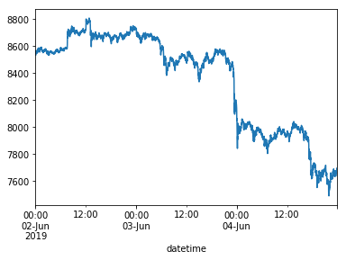
<matplotlib.axes._subplots.AxesSubplot at 0x1211da748>
Date slicing
Now that we've successfully set the 'datetime' column as the DataFrame index, we can also slice that index using date strings! If we want to only use a data subset containing 1 day of trading data (= 1440 K-line ticks in this data set), for example on 2019-06-02, then we simply pass the date string as an argument, like so:
df_20190602 = df['2019-06-02']
df_20190602.tail()
| open | high | low | close | volume | |
|---|---|---|---|---|---|
| datetime | |||||
| 2019-06-02 23:55:00+00:00 | 8725.31 | 8728.61 | 8721.67 | 8725.43 | 10.443800 |
| 2019-06-02 23:56:00+00:00 | 8725.45 | 8729.62 | 8720.73 | 8728.66 | 10.184273 |
| 2019-06-02 23:57:00+00:00 | 8728.49 | 8729.86 | 8724.37 | 8729.10 | 10.440185 |
| 2019-06-02 23:58:00+00:00 | 8729.05 | 8731.14 | 8723.86 | 8723.86 | 9.132625 |
| 2019-06-02 23:59:00+00:00 | 8723.86 | 8726.00 | 8718.00 | 8725.98 | 9.637084 |
As you can see on the .tail()output, the last DataFrame row of the newly created df_20190602 DataFrame is 2019-06-02 23:59:00, and the df_20190602 DataFrame only contains 1440 rows of data in total:
df_20190602.shape
(1440, 5)
In case we want to create a DataFrame containing a multiple day window subset, we also add a stop date to the date string slice, like so:
df_20190602_20190603 = df['2019-06-02':'2019-06-03']
df_20190602_20190603.tail()
| open | high | low | close | volume | |
|---|---|---|---|---|---|
| datetime | |||||
| 2019-06-03 23:55:00+00:00 | 8170.31 | 8178.48 | 8162.61 | 8169.20 | 46.913377 |
| 2019-06-03 23:56:00+00:00 | 8169.24 | 8175.39 | 8159.00 | 8161.52 | 44.748378 |
| 2019-06-03 23:57:00+00:00 | 8161.16 | 8161.17 | 8135.94 | 8146.69 | 65.794209 |
| 2019-06-03 23:58:00+00:00 | 8146.58 | 8153.00 | 8137.38 | 8140.00 | 43.648000 |
| 2019-06-03 23:59:00+00:00 | 8140.00 | 8142.80 | 8100.50 | 8115.82 | 185.607380 |
df_20190602_20190603.shape
(2880, 5)
Nota bene: It's important to note that - unlike on "regular" (index) slicing, - when using date string slicing in pandas both lower and upper boundaries are inclusive; the data being sliced includes all 1440 data rows from June 3, 2019.
Time slicing using .between_time()
What if we want to slice all 1-minute candles which happened one a specific day (e.g. on 2019-06-02) between a specific time interval, for example between 14:00 UTC and 15:00 UTC? This we can accomplish using the .between_time() method.
As arguments, we pass the arguments start_time, end_time, and we specify include_end=False so that the end_time is non-inclusive (if we wouldn't, our new sub-set would include 61 instead of 60 1-minute ticks).
df_20190602_1h = df_20190602.between_time('14:00', '15:00', include_end=False)
df_20190602_1h.tail()
| open | high | low | close | volume | |
|---|---|---|---|---|---|
| datetime | |||||
| 2019-06-02 14:55:00+00:00 | 8665.71 | 8669.50 | 8663.66 | 8667.24 | 11.401655 |
| 2019-06-02 14:56:00+00:00 | 8668.06 | 8670.90 | 8664.87 | 8667.07 | 11.358376 |
| 2019-06-02 14:57:00+00:00 | 8667.07 | 8670.90 | 8664.96 | 8669.96 | 15.915794 |
| 2019-06-02 14:58:00+00:00 | 8670.00 | 8673.37 | 8669.46 | 8672.73 | 11.153078 |
| 2019-06-02 14:59:00+00:00 | 8672.72 | 8672.72 | 8663.57 | 8663.59 | 9.850304 |
df_20190602_1h.shape
(60, 5)
Some basic pandas statistic operations (including gaining some real-life Binance BTCUSDT statistical insights while we're at it)
.max()
To retrieve and return the maximum value of a selected DataFrame column, pandas provides the .max() method. First we select the column we want to inspect, and run the .max() method on that, like so (on the original df DataFrame we began with):
df['open'].max()
8808.82
.idxmax()
And in order to return the DatetimeIndex on which the maximum value (within the selected range, or in this case the total dataset) occurred, use .idxmax():
df['open'].idxmax()
Timestamp('2019-06-02 12:48:00+0000', tz='UTC')
Interestingly, if we check .idxmax() on the "volume" data, '2019-06-03 23:22' is returned. If we look back at the price plot, we can visually spot a "flash crash" of BTC price happening over the course of a few minutes, in which Bitcoin price dropped from about 8500 to around 7800!
The trading volume of Bitcoin (mostly sells) on Binance happening in just one minute ('2019-06-03 23:22' UTC) was almost 950 Bitcoin!
df['volume'].idxmax()
Timestamp('2019-06-03 23:22:00+0000', tz='UTC')
df['volume'].max()
949.563225
.min()
As you have probably guessed, in order to return the minimum value we use the .min() method:
df['open'].min()
7490.2
.idxmin()
Similarly, in order to return the DatetimeIndex on which the minimum value occurred, run .idxmin():
df['open'].idxmin()
Timestamp('2019-06-04 22:00:00+0000', tz='UTC')
.mean()
The mean value of a specific series is found by using the .mean() method. Using our entire 3-day dataset, we find that the mean price of Bitcoin between June 2, 2019 and Jun 4, 2019 was 8354.03:
df['open'].mean()
8354.033474537022
Having found already that the maximum amount of Bitcoin traded (within our 3 day range) in just minute was about 950 Bitcoin, let's check the average minute trading volume as well:
df['volume'].mean()
34.18334428472222
.sum()
Suppose we want to compute the total trading volume which happened on our entire 3-day DataFrame, then we can do so easily using the .sum() method on the df['volume'] column, like so:
df['volume'].sum()
147672.04731
This number is indeed correct, which we can check by multiplying the amount of 1-minute ticks (4320) in our dataset by the mean 1-minute volume we just returned:
4320 * 34.18334428472222
147672.04730999997
.describe()
The basic statistical values we've been using thus far (which of course can be used on more complex DataFrame operations, which we'll discuss in the forthcoming tutorial episodes), we can also output on (a selection of) the entire DataFrame using the .describe() method:
df.describe()
| open | high | low | close | volume | |
|---|---|---|---|---|---|
| count | 4320.000000 | 4320.000000 | 4320.000000 | 4320.000000 | 4320.000000 |
| mean | 8354.033475 | 8359.921905 | 8347.543243 | 8353.818926 | 34.183344 |
| std | 358.395024 | 357.338897 | 359.911089 | 358.538551 | 54.520356 |
| min | 7490.200000 | 7533.430000 | 7481.020000 | 7494.110000 | 1.351415 |
| 25% | 7985.045000 | 7990.270000 | 7979.205000 | 7984.997500 | 11.114809 |
| 50% | 8519.605000 | 8524.985000 | 8513.490000 | 8518.845000 | 19.566122 |
| 75% | 8661.080000 | 8666.992500 | 8656.007500 | 8661.200000 | 35.273851 |
| max | 8808.820000 | 8814.780000 | 8805.850000 | 8809.910000 | 949.563225 |
What did we learn, hopefully?
Hopefully you've learned the difference between regular integer index values and DateTimeIndexes, and why and how those are useful on Time Series analysis using pandas.
Thank you for your contribution @scipio.
After reviewing your tutorial we suggest the following points listed below:
Again: The curriculum section becomes very large at the beginning of the tutorial. Maybe you should put it at the end of your tutorial.
In your construction of your text for the tutorial, always do in the third person. This is consistent.
Improve the structure of the tutorial, the tables become a bit poorly formatted.
Thank you for your work in developing this tutorial.
Looking forward to your upcoming tutorials.
Your contribution has been evaluated according to Utopian policies and guidelines, as well as a predefined set of questions pertaining to the category.
To view those questions and the relevant answers related to your post, click here.
Need help? Chat with us on Discord.
[utopian-moderator]
Thx again for reviewing! I've used your suggestions on the (now) published ep.032, but please keep in mind that I have no control over the
font-sizevalues of the tabular data on the Condenser frontends; the<style>elements Jupyter Notebooks output "I've had to strip away in order to post via Condenser.Thank you for your review, @portugalcoin! Keep up the good work!
Thank you scipio! You've just received an upvote of 8% by artturtle!
Learn how I will upvote each and every one of your posts
Please come visit me to see my daily report detailing my current upvote power and how much I'm currently upvoting.
Thx @artturtle!
Hi @scipio!
Your post was upvoted by @steem-ua, new Steem dApp, using UserAuthority for algorithmic post curation!
Your post is eligible for our upvote, thanks to our collaboration with @utopian-io!
Feel free to join our @steem-ua Discord server
Thx @steem-ua!
Hey, @scipio!
Thanks for contributing on Utopian.
We’re already looking forward to your next contribution!
Get higher incentives and support Utopian.io!
Simply set @utopian.pay as a 5% (or higher) payout beneficiary on your contribution post (via SteemPlus or Steeditor).
Want to chat? Join us on Discord https://discord.gg/h52nFrV.
Vote for Utopian Witness!
Thx @utopian-io!
[Bleep! Bleep!]Hi, @scipio!
You just got a 0.05% upvote from SteemPlus!
To get higher upvotes, earn more SteemPlus Points (SPP). On your Steemit wallet, check your SPP balance and click on "How to earn SPP?" to find out all the ways to earn.
If you're not using SteemPlus yet, please check our last posts in here to see the many ways in which SteemPlus can improve your Steem experience on Steemit and Busy.